Graphical User Interface

The Graphical User Interface (GUI) is the component of FullProfAPP that controls the functionality of the program. It is implemented using PyQt5, a Python wrapper for Qt, which is a popular C++ library for GUI development. The main window of FullProfAPP looks like this (Fig. 2).

Fig. 2 Main window of FullProfAPP. The toolbar (red), the graphics area (blue), the terminal and materials area (green), and the protocols and file system area (purple).

The colored sections in (Fig. 2), are resizable by dragging the splitters that exist in between.

Toolbar

The toolbar contains four menus: File, Pattern, Materials, View, and Help that contain the following actions:

• File

  • Select Project Folder: Select the work directory for the project

  • Save: Click or press Ctrl+S to save the current state of the application

  • Save As: Click to save the current state of application to a file

  • Load: Load application state from a file

  • Clear Work Directory: Delete all the data generated by the program in the working directory

  Note

  The loading/saving of the application state is done through an INI file with a .fpapp extension, which is registered in your OS upon installation. These files can be loaded directly from the GUI or by double clicking on the file itself.

  Warning

  The .fpapp files do not save all the information about the previous session, instead they only save the internal state variables of the interface. This keeps the files lightweight because they do not have to save all the raw data coming from the execution of FullProf. However, some of those state variables refer to the location of the raw data in the OS. This means that the loading process will fail if the user moves the files from their original locations. In this case, FullProfAPP will try again to find the data assuming that the .fpapp file was saved in the working directory

  

  Fig. 3 Folder structure assumed by FullProfAPP

• Pattern

  • Import Pattern: Launch a dialog window where experimental data is loaded:

    • Pattern File: Load diffraction pattern files. Check the From (.buf) box to load patterns from an external buffer that contains the location of the patterns ordered in a column.

    • File Format (.*):

      • xys/xye/xy: XY column format (Ins = 10)

      • free: Free format (Ins = 0)

      • socabim: Format generated by Socabim software (Ins = 9)

      • xrdml: XML format (Ins = 13)

      • D1A/D2B (ILL): ILL detectors (Ins = 6)

      • D1B/D20 (ILL): ILL detectors (Ins = 3)

      • DMC (PSI): DMC instrument from Paul Scherrer Institute (Ins = 8)

    • IRF File: Load Instrumental Resolution Function (IRF) files.

    • Format (Res): Select the format of the IRF file (Res in the PCR files)

    • Wavelength (A): Input the infomation about the radiation wavelength. You can use some predefined values in the box that is located to the right.

    • Radiation: X-Rays or CW Neutrons

    • Geometry:

      • DEBY: Debye-Scherrer geometry (Ilo = -2)

      • BRAG: Bragg-Brentano geometry (Ilo = 0)

      • SYNC: Synchrotron Debye-Scherrer geometry (Ilo = 3). The value of the polarization will be requested.

      • PSD: Flat plate PSD geometry (Ilo = 1). The value of the incident fixed angle (in degrees) will be requested.

      • TRMB: Transmission bisecting geometry (Ilo = 2)

      • TRMF: Transmission fixed geometry (Ilo = 4). The value of the incident angle (in degrees) with respect to the sample normal will be requested.

    • Options: Set-up multi-pattern refinements. When clicking on you will see a placeholder (Pattern Group #N) appear.

    • Add Files/Clear Files: When all the above mentioned fields are complete, click Add Files to fill the selected Pattern Group #N placeholder. Click Clear Files to delete all entries.

    

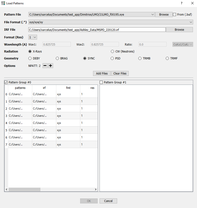
    Fig. 4 Import Pattern dialog window.

    Note

    • Support for Time of Flight (TOF) neutrons will come in future versions of the program

    • When providing an IRF file FullProfAPP will inspect it in search of keywords that provide instrumental information such as, WAVE, THRG, GEOM, etc. In case the keywords are present in the file, the corresponding options will be disabled in the dialog window. Otherwise, you will have to include the appropriate information in order to proceed.

    • You can select the order in which you load the patterns into FullProfAPP by sorting the pattern files in you OS’s explorer dialog when clicking Browse. This can be useful if you are refinining patterns sequentially and several phases appear overlapped. You can select the patterns where the different phases are more clearly distinguished, and run your sequential refinements forwards and backwards such that you have better starting guesses when dealing with highly overlapped reflections.

    Warning

    • It is mandatory to provide an IRF file in order to work with FullProfAPP. The app will not allow you to proceed otherwise.

    • All Pattern Group #N placeholders must contain the same number of entries

    • All loaded patterns in their respective Pattern Group #N placeholders must have the same radiation type, diffractometer geometry, and wavelength

• Automatic Background: Extract background points for the loaded patterns using the Asymmetric Least-Squares (AsLS) smoothing method as implemented in the PRISMA software

• Peak Detection: Detect peak positions and intensities

• Edit Background: Toggle to enter in manual background editing mode

• Edit Peaks: Toggle to enter in manual peak editing mode

• Export Background: Exports background points as a XY column text file

• Export Peaks:

  • Free Format: Export peaks positions, intensities, and background in a three column file with .aps file extension

• Materials

  • Search in Remote Database: Filter crystallographic phases from the COD, download the corresponding CIF files into the working directory, and load them in the app.

  • Search in Local Database: In the case the CIF files are already available on your local machine, you can select the folder in which they are located and directly load them into the app.

• View

  • Current (.prf): Plot the profiles resulting from the most recent refinement process inside the graphics area (see Fig. 2)

  • Select (.prf): Plot the refinement profiles from any other file with a .prf extension

  • Current (WinPLOTR): Plot the most recent refinement profiles using WinPLOTR

  • Select (WinPLOTR): Plot the refinement profiles from any other file with a .prf extension using WinPLOTR

  • Current Results (.sum/.mic): Plot a summary of the last results obtained from the refinement process inside the graphics area (see Fig. 2)

  • Select Results (.sum/.mic): Same as above but selecting any folder in your system

  Note

  In order to use WinPLOTR, it must be available and visible to FullProfAPP, so make sure to follow the Installation process properly.

• Help

  • Online Manual: Click on it to open the manual for FullProfAPP in your default internet browser

  • About: Click on it to get current version of FullProfAPP

Graphics Area

The graphics area contains the functionality for the visualization of the experimental data and the refinement results. It contains tabbed sections that become available at different stages of the analysis.

• Exp. Data: This tab is always visible and contains the experimental pattern plots, the detected background, and peak positions and intensities (if requested).

• Prf Data: It plots the experimental profiles superimposed to the calculated total profiles, individual phase’s profiles, difference plots, and the hkl reflections.

• Summary: Visualizes model parameters resulting from the refinements. The parameters are selected with a checkable tree that allows you to select the parameters of interest.

  • Export Data: This button allows to export a text file of the contents of the graph as XY columns.

  • Check All: This button checks and unchecks all of the items in the checkable tree to facilitate exporting all of the data.

  

  Fig. 5 Widget for visualizing the refinement results. The values of the gaussian strain broadening are shown along with their standard deviations.

Graphics Toolbar

Note that on top of the plotting region in Fig. 2 (blue region), there is an additional toolbar which is meant to help you navigate between all the loaded patterns and refined profiles with the following actions.

• Pattern List: This combo box lists all loaded patterns. You can click on any item on the list to change the focus and visualize the associated pattern and results (if any). The / arrows can be clicked to change the focus to the previous/next item in the list.

• PATT: / arrows change the focus to the different patterns that will be considered in a single refinement. They will be enabled if the patterns are loaded to perform multi-pattern refinements.

• Pattern Checks: This button spawns a menu that contains a table with all the pattern identifiers. Each cell on the table contains a checkable box. Those items that are set as checked will be selected for subsequent refinements, while those marked as unchecked will be ignored.

• Contour Plot: Click to plot all of the loaded patterns.

  • Contour: Plot the contour of the patterns

  • Surface: Plot the 3D surface of the patterns

Note

The Pattern Checks context menu works as a selector for refinement jobs. When a batch of files are loaded in a single pattern group (Import Pattern), you will see all pattern identifiers appear ordered in rows. When adding more pattern groups and loading another batch of pattern files, you will see that pattern identifiers show additional columns. Any row that contains at least one checked cell is set to be refined. Thus, rows indicate separate refinement jobs. On the other hand, columns indicate that a single refinement will be carried out simultaneously on several patterns (the least squares fitting process will consider more than one experimental pattern).

Fig. 6 Pattern checks context menu, showing a dummy example where a batched multi-pattern refinements is performed with XRD and NPD data simultaneously. Here, we loaded eight patterns, but we organized them in four rows and two columns. Looking at the checked boxes, the rows 2, 3, and 4, have been selected for further refinements. Where row 3 will exclude any contribution from the pattern in the first column, and viceversa for row 4.

Interacting with Graphs

You can interact with graphs in the following way

• Zoom: Mouse Left Drag

• Reset view: Mouse Left Click

• Move view: Press keys

• Extra options: Ctrl + Mouse Right Click to spawn a menu with additional options (change graph properties, save plots, etc.)

If the Pattern List <toolbar> combo box is selected you may use the the arrow keys to swiftly scroll through the loaded patterns (this applies to every combo box in the app).

Additionally, you can edit background and peaks points. For this you must first toggle the Edit Background or Edit Peaks modes.

• Ctrl + Mouse Left Click: Select the point that is closer to the cursor. The point will be highlighted in red

• Ctrl + Mouse Left Drag: Select all the points within the designated area

• Shift + Mouse Left Click: Add point in cursor positions

• Mouse Left Click: Reset selection

• Delete: Delete selected points

When working with contour plots you have two additional options.

• Shift + Mouse Wheel: Vary the top level of the colorbar

• Ctrl + Mouse Wheel: Vary the bottom level of the colorbar

Terminal and Materials area

The area in Fig. 2 (green region) contains four tabs

• Terminal: It displays information about the programs that are run in the background, such as fp2k and CIFs_to_PCR. It is always visible and contains the following buttons:

  • Kill: Immediately stops the execution of the current process

  • Clear: Clear the displayed text

  Note

  The Kill button is useful when an abnormal stop of the background processes happen. In principle, FullProfAPP handles this automatically, but you can use it in case the application hangs out completely.

• Queried Materials: This tab includes a table that contains crystallographic information about the CIF files loaded using the materials menu, such as, identifiers, formula, space group, cell parameters, etc.

  • Double Mouse Left Click: If clicked on the identifier column, edit the identifier names. Changes will also apply to the original CIF files saved in the OS.

  • Mouse Left Click + Drag/Ctrl/Shift: Select entries from the table

  • Delete: Delete selected entries from the table (not the CIF files themselves)

  • Filter: Editable text prompt to filter table entries by coincidence.

  • Submit Selection: The selected entries are saved into the Selected Materials tab, which are then going to be used in subsequent refinements

  • Simulate Selection: Launch a FullProf simulation of the selected phases using the focused experimental pattern as a reference.

  

  Fig. 7 Queried Materials tab.

• Selected Materials: This tab includes a table containing the entries that where selected from the Queried Materials table. The Double Mouse Left Click, Mouse Left Click + Drag/Ctrl/Shift, and Delete functionallities are the same as in Queried Materials.

• Results: After a successful run of a refinement process, this tab becomes visible. It contains a summary with basic information about the phases that were refined.

Protocols and File System area

The area in Fig. 2 (purple region) contains two tabs

• File System: Shows the folder and file structure of the working directory. A context menu appears when using Mouse Right Click with many options

  • Show File: Show the contents of the selected file

  • Rename: Rename the selected item.

  • Copy (Ctrl+C): Copy the selected items from the File System tree

  • Paste (Ctrl+V): Paste the copied items into the File System tree. Changes will be reflected on your OS

  Additionally you may use the Delete keyboard button to delete the items and Mouse Double Right Click to open the file or folder with the default OS application (Explorer, VESTA, Notepad++,…)

  Warning

  • You cannot copy/paste from the clipboard directly onto the File System tree. Copy/Pasting is just internal to the File System tree.

  • Renaming or Deleting certain items may cause problems because you might be manipulating data that FullProfAPP is using for refinements and visualization and you will receive warning messages from the app. Alternativaly, the app will not allow you to eliminate critical files from the File System. Although you might still do it directly from the OS explorer.

  • Opening files with the Mouse Double Right Click requires you to previously set the default application for a given file extension. In Linux, this is possible to do using the desktop GUI. If you are working directly from the terminal you will need to set the neccessary MIME Types for the extensions using the xdg utilities that most likely come already installed in your distro. Here some materials to read:

    • ArchLinux Wiki: https://wiki.archlinux.org/title/XDG_MIME_Applications

    • More links: https://www.rigacci.org/wiki/doku.php/doc/appunti/linux/tux/mimetype

• Protocols: Contains expandable buttons that contain parameter fields and utilities to run the corresponding refinement protocols. The program implements three options

  • Full-Profile Phase Search Protocol

  • Automatic Refinement Protocol

  • Manual Refinement

The following sections provide detailed information about these protocols

Full-Profile Phase Search Protocol

This protocol implements the full-profile search-match algorithm originally devised by L. Luterotti, et. al.. It takes all the CIF files corresponding to the entries of the Selected Materials table and runs a series of refinements using fp2k in order to determine which phases are most likely to be present in your sample(s). The widget that controls the execution of this protocol contains the following options:

Fig. 8 Full-Profile Phase Search Protocol window.

• Background Combo: It contains a list with three options.

  • Linear Interpolation: The background will be extracted from a linear interpolation of the background points extracted with the Automatic Background option.

  • Chebyshev: The background is fitted to a Chebyshev polynomial expansion. The starting guess for the polynomial coefficients is done using the background points extracted with the Automatic Background option. An additional parameter must be provided:

    • Order: An integer number specifying the order of the Chebyshev polynomial expansion

  • Fourier Filtering: The background is calculated using the Fourier filtering method. Two additional parameters must be provided

    • Window: The size of the window used, the larger its value the smoother the background (minimum Npoints/6 where ‘Npoints’ is the number of data points of the patterns)

    • Cycle: An integer value specifying the frequency in which the Fourier filtering is applied (once every Nth convergence cycles)

The following three parameters control the refinement workflow based on phase weight fractions

• f_R0: If phase weight fractions fall bellow f_R0, they are ignored in the subsequent refinements

• f_R1: If phase weight fractions fall above f_R1, the instrument correction parameters and unit cell parameters are refined

• f_R2: If phase weight fractions fall above f_R2, the overall isotropic temperature factors and the crystallite size and strain broadening parameters are refined.

The parameters that control the refinement process are given by

• NCY: Number of convergence steps for the refinement

• Ste: Reduce the experimental patterns’s data size by taking one data point every Ste points

• R_at: Relaxation factor for atomic parameters, the lower the value, the smoother the convergence, at the cost of needing more NCY cycles

• R_an: Relaxation factor for anisotropic displacements

• R_pr: Relaxation factor for profile parameters

• R_gl: Relaxation factor for global parameters

Additionally, the Scan Step Parameters contain fields that define the Figure of Merit (FoM) that is used to rank the phases that provide the best fit for the experimental patterns:

• FoM_a: Increasing its value favors phases whose initial cell volumes are close to the refined ones

• FoM_b: Favor low scattering phases

• FoM_c: Penalize phases with low average apparent crystallite sizes

• FoM_d: Penalize phases with high average maximum strains

Note

The explicit formula for the FoM, which is adapted to work with FullProf is given as

\[FoM^p = \left [ \frac{1}{R_{wp} + a v_0^p |\frac{1}{v_r^p} - \frac{1}{v_0^p}|} + b (100.0 - f_r^p) \right ] \left (1 + \frac{c}{\langle D^p \rangle} + d \langle \varepsilon^p \rangle \right )^{-1}\]

Where \(R_{wp}\) is the weighted profile factor, \(v_p\) (\(v_0\)) is the refined (initial) cell volume, \(f_r\) is the weight fraction, \(\langle D \rangle\) is the average apparent crystallite size, and \(\langle \varepsilon \rangle\) is the average maximum strain. Here, the superscript \(p\) indicates that the values correspond to the phase that is being evaluated in the scanning process.

• f_S1: If a phase weight fraction falls bellow f_S1 during the scanning process, it is directly eliminated from the candidate list

The Quantification Step contains two additional parameters

• f_S0: If a phase weight fraction falls bellow f_S0 during the quantification process, it is eliminated from the list of detected phases

• Similarity Index: Calculates the DeGelder similarity index. Two phases are considered equal if the calculate value is larger than the given value (range \([0.0, 100.0]\))

Finally, the excluded regions define the regions in \(2\theta\) that are not considered in the refinement process.

• Min/Max: Define the excluded \(2\theta\) range.

• / buttons: Remove/Add the defined excluded regions to the list. The excluded regions can also be removed by clicking on the list items and pressing Delete

• / buttons: Select the pattern for which the excluded regions are set. This option is enabled for multi-pattern refinements.

• Select any item representing an excluded region and press Delete to remove it

Each time you run this protocol a new directory will be created named FPSEARCH### where the # is a number that depends on how many directories exist with the same prefix (the first time you run this protocol the results will be saved in the FPSEARCH000 folder, then FPSEARCH001, and so on).

Automatic Refinement Protocol

This is the most general way of using FullProfAPP. This protocol window allows you to handle large series of patterns and running your refinements with flexible, user-defined, refinement sequences. You can also run sequential refinements, by running the same refinement sequences through the whole pattern series, taking the outputs from the previous pattern’s refinement as inputs for the next one. The protocol window is divided into the Patterns and Workflow sections.

Fig. 9 Automatic Refinement Protocol window.

• Patterns: Is used to setup the refinement data. Particularly, it links all checked patterns with FullProf’s PCR input files. It contains the following widgets:

  • Pattern List: It shows a list of pattern names similar to the one shown in the toolbar area. The difference is that only those patterns that have been selected for refinement (checked) appear in the list

  • Load .pcr(s): Load an external PCR input file for the patterns appearing in the Pattern List

  • : Generate a PCR input file for the currently focused item in the Pattern List using CIFs_to_PCR. The PCR files will contain all the phases appearing in the Selected Materials table.

  • : Delete the PCR file associated with the currently focused item in the Pattern List

  • : Generate PCR input files for all items in the Pattern List containing the phases appearing in the Selected Materials table

  • : Delete all PCR files associated to the items in the Pattern List

  • Pattern Phases: Shows a tree view of the phase identifiers that are linked to the items in the Pattern List

  Note

  • When generating a PCR file using the or buttons, FullProfAPP will read the entries in the Selected Materials table and use those to build the PCR file. If some of the entries in the Selected Materials table are highlighted, only those will be used to build the PCR file. On the contrary, if there are no ongoing selections, all entries will be used.

  • If a PCR file is already loaded for the given pattern, only the phases that are not already included are added from the Selected Material table. Thus, the results of the current refinements are saved. This allows the user to add new phases after the refinement process has already started.

  • The PCR files will be generated with the background points of the corresponding patterns as obtained with the Automatic Background option.

  Warning

  At this point it is worth giving a word of caution for those users that wish to load their external PCR files using the Load .pcr file(s) button. FullProfAPP is not built as a complete wrapper of FullProf, and it is important to acknowledge that it has certain limitations when handling more advanced cases that require specialized knowledge of FullProf, such as, symmetry modes, magnetic structure refinements, single crystal diffraction, etc. Instead, FullProfAPP should be viewed as a high abstraction layer for FullProf that automates, extends functionality for high-throughput and operando data treatment, and helps ease the entrance barrier for more novice users.

  In addition, press Mouse Right Click in the Pattern Phases tree items to spawn a context menu with extra options:

  • Background options:

    • Load on Selection: Replace the background on the selected tree items with the ones appearing on the Graphics Area, or with an external background file

    • Load on Sequential: In a sequential refinement, instead of using the background parameters from the previous pattern’s PCR file as input for the current refinement, use the background appearing on the Graphics Area for the same pattern.

    Note

    The Load on Sequential option is only visible if two conditions are met. (i) The sequential refinement mode is activated, and (ii) the backgrounds for all the patterns that will be refined sequentially are available (Automatic Background).

• Workflow:

  • Background Combo: It contains a list with three options.

    • Linear Interpolation: The background will be extracted from a linear interpolation of the backgroung points specified in the PCR file.

    • Chebyshev: The background is fitted to a Chebyshev polynomial expansion. An additional parameter must be provided:

      • Order: An integer number specifying the order of the Chebyshev polynomial expansion

    • Fourier Filtering: The background is calculated using the Fourier filtering method. Two additional parameters must be provided

      • Window: The size of the window used, the larger its value the smoother the background (minimum Npoints/6 where ‘Npoints’ is the number of data points of the patterns)

      • Cycle: An integer value specifying the frequency in which the Fourier filtering is applied (once every Nth convergence cycles)

    Warning

    When using the different background modes there are some rules in the way FullProfAPP handles them.

    • The Linear Interpolation option will not make any changes if the underlying PCR already contains background points that define a linear interpolation for the background. However, when the underlying PCR file contains Chebyshev coefficients instead (nba = -5), FullProfAPP will transform this polynomial expansion back into a set of discrete background points (30 by default).

    • Similarly, the Chebyshev option will try to fit a Chebyshev polynomial expansion of a given order only if the underlying PCR contains background points defining a linear interpolation.

    • When the underlying PCR is defining a Fourier Filtering of the background, you will not be able to switch back to the Linear Interpolation or Chebyshev background modes. In this case, use the Load on Selection option to reload a background extracted with the Automatic Background options.

  • Refinement Parameters: Contains a checkable parameter tree. The items on the tree represent refinable parameters that are updated each time a new PCR file is loaded in the Pattern Phases tree. Expanding the tree items you will see the different phases and crystallographic sites to which the refinements will be applied. The checked items will be selected as part of the refinement workflow by clicking the button. Multiple tree items can be selected with Ctrl/Shift + Mouse Left Click. Mouse Right Click on the selected items to access more refinement options:

    • New Linear Restraint: Impose a restraint (soft-constraint) between two or more parameters. The fitting procedure will try to meet the condition that the linear relation between the selected parameters, scaled by user-defined coefficients, is equal to a value with a given tolerance (also defined by the user). Follow this tutorial for more details. Once a linear restraint is added, an extra item named Restraint # will appear in the menu, signalling that the restrain is set to be part of the workflow. An indefinite amount of restraints can be stacked. In order to delete them, hover to the menu item with your mouse and press Delete.

    Note

    FullProfAPP imposes several conditions on the application of linear restraints. If the conditions are not met, the app will hide the option from the user.

    • The selected parameters must be checked in the parameter tree

    • Cannot select a tree item which itself contains other sub-items

    • Restraints that involve cell parameters are not included

    • New Constraint: Define a hard-constraint between several parameters. Unlike linear restraints, the constrained parameters are forced to change according to the coefficients given by the user. For example, if two parameters are related by coefficients 1.0 and -1.0, any increase in the value of the former must be matched with an equal decrease of the value of the latter. Once a constraint is added, and extra item named Constraint # will appear in the menu. Hover your mouse and press Delete to remove the constraint.

    Note

    Additional conditions for constraint options

    • A single parameter cannot be involved in two different sets of constraints

    • The cell parameters of a single phase can be constrained to be equal for the case of multi-pattern refinements. This is achieved through the PEQU_pat directive in the COMMANDS/END COMMANDS block of the PCR files.

    • New Limit: Define a limit for a given parameter. The Low Limit and High Limit line edits mark the allowed range of values that the given parameter can take. The Boundary can take two values 0 or 1, indicating that the refinement of the parameter is stopped if the parameter reaches a certain limit (0) or the parameter has periodic boundary conditions (1) (for example in the case of atom coordinates). The Coefficient is a real number that define the rate of change of the parameter (same as the New Constraint and New Linear Restraint options).

    • Profile Matching (Constant Scale Factor): The selected phase will be treated in profile matching mode using the LeBail fitting method.

    • Profile Matching (Constant Relative Intensities): The selected phase will be treated in profile matching mode. In this case, the relative intensities of the reflections are kept constant, meaning that the scale factors can be optimized. When activating this option, the program will ask you to feed a structure factor HKL file (with .hkl extension).

    Warning

    Keep in mind that when activating the Profile Matching mode you should never refine site parameters (atomic positions, temperature factors, occupations). In case the Profile Matching (Constant Scale Factor) is activated, you should also leave the scale factors of the selected phases untouched. FullProfAPP will warn if you try to set up any option that is bound to fail, but will not stop the execution of the workflow.

  • Duplicate Sites: Duplicate the selected site(s) in the parameter tree by giving it new labels and atom types

  • Workflow tree: The panel to the right of the Refinement Parameters tree shows the refinement workflow that is built by clicking the button after checking the refinement parameters of interest. The workflow is built as a list where each refinement step (named Step #) is added to the previous one. Expanding the tree items will show you all the information that is going to be included in the PCR files for the refined (fixed) parameters under the VARY (FIX) tags. The refinement of each checked pattern will be done by following these steps from first to last.

    • Load Workflow: Click Mouse Right Click to load a workflow from an external file

    • Save Workflow: Click Mouse Right Click to save the current workflow to an external file

    Warning

    (The workflow load/save feature is prone to fail)

    We remind the reader that FullProfAPP interfaces with FullProf through input/output files. Thus, FullProfAPP makes heavy use of the phase name identifiers and site labels to make distinctions between different phases and crystallographic sites (without performing any further crystallographic operations to check for equivalent phases or sites). Which means that it is at the user’s discretion to name these phases and crystallographic sites uniquely for FullProfAPP to work correctly. This is important to mention because the workflow files, which are formated as JSON text files and contain all the information about the refinement workflows, will be saved in your OS to be later loaded by FullProfAPP. Thus, if phase and site labels are not correct, or if you mistakenly load a workflow that does not belong to the system you want to study, things might go wrong. For example:

    • The workflow files contain phase entries that do not match: When loading a workflow file, the identifiers (phase names) of the different crystal structure models do not match with any of the identifiers you loaded using the Load .pcr(s) or the and buttons. In this case FullProfAPP will not allow you to continue loading the workflow.

    • The workflow files contain site labels that do not match: Similarly, it is possible that for a matching identifier (existing in both the workflow file and loaded data), the workflow file refers to a crystallographic site with a label that does not match with any other crystallographic site label you loaded. Again, FullProfAPP will not allow you to continue loading the workflow.

    • The loaded data contains more phase entries than the workflow file: It can also happen that you load more phases than those included in the workflow file. In this case FullProfAPP will warn you and let you continue if you agree. This is risky, because the workflow will only take effect on a subset of all the parameters you loaded, ignoring the rest. Meaning that at each refinement step, you might still be refining some additional parameters that are not explicitly included in the workflow, specially when using an external PCR file.

    • For matching phase entries, the loaded data contains more sites than the workflow file: Similar to the previous case, for a phase identifier that is included in both the workflow file and the loaded data, it may happend that the loaded data contains more sites than the workflow file. Thus, the same considerations of the previous point apply.

    • You loaded a different JSON file that has nothing to do with a workflow: You may mistakenly load a completely unrelated JSON file onto the program. In principle, you should see an error message appear. In the worst case scenario, the workflow is succesfully loaded and there are not error messages, meaning that FullProfAPP will fail at some future step. (Future versions of FullProfAPP will make a more exhaustive validation of the workflow files to avoid any dodgy errors)

  • Excluded Regions: See excluded regions

  • Fix Elements: Write the symbols(s) of the element(s) whose sites you want to exclude from the refinement.

  Note

  The symbols must coincide with the element symbols of the PCR files, an must be given a blank-space separation. The program includes a FIX_SPC directive in the COMMANDS/END COMMANDS block of the PCR files

Additionally the fields that control the execution of FullProf are the following:

• NCY: See control parameters

• Ste: See control parameters

• R_at: See control parameters

• R_an: See control parameters

• R_pr: See control parameters

• R_gl: See control parameters

• Sequential Mode: When checked, FullProfAPP assumes that the loaded patterns belong to a series in which the refinement parameters of a given pattern is related to the refinement of the previous one. The user can interact with the protocol window as usual but the way the samples are refined changes.

  • More patterns are refined: In contrast to the normal behavior, where only the patterns that are checked are refined, all patterns between the first and last checked patterns are considered. If only a single pattern is checked then all patterns between this and the last one are refined.

  • Sequential run: FullProfAPP connects the initially built PCR files between the abovementioned checked patterns and uses the refinement parameters that resulted from the previous pattern as inputs for the next one.

Each time you run this protocol a new directory will be created named FPAUTO### or FPSEQ### (depending if the Sequential Mode is activated or not). Here the # is a 3-digit number that depends on how many directories exist with the same prefix (the first time you run this protocol the results will be saved in the FPAUTO000 folder, then FPAUTO001, and so on).

Note

Whether the Sequential Mode is activated or not, FullProfAPP monitors the weight fractions of the constituent phases along the refinement process. If the weight fraction of any particular phase falls below a threshold of 2%, it will be ignored for the rest of the workflow. This allows to have robust refinement that avoid divergences with parameters that are hard to refine in minority phases.

Manual Refinement

The Manual Refinement window allows you to interact with the PCR input files in the same way you would with a text editor. Similar to the previous section you can find the following:

• Patterns

  • Pattern List: See patterns

  • Load .pcr(s): See patterns

  • : See patterns

  • : See patterns

  • : See patterns

  • : See patterns

When loading the PCR files the panel below will spawn the contents of the files formatted in tables that contain editable cells. Some of those cells are kept fixed while others react automatically to the user’s changes, such as number of background points (Nba), number of excluded regions (Nex), number of sites (Nat), etc. Some tables also contain checkable boxes that activate additional refinement parameters. Among the supported options we can find:

• Micro-absorption parameters

• Bond-Valence sum parameters

• Phase dependent \(2\theta\) shifts

• Anisotropic thermal parameters

• Anisotropic strain broadining plus lorentzian strain broadening: Concrete mode set-up automatically by reading the specific Laue class of the phase, which is inferred from the space group.

• Anisotropic size broadening with spherical harmonic expansion: Concrete mode set-up automatically by reading the specific Laue class of the phase, which is inferred from the space group.

The words of caution still apply here. While the Manual Refinement window allows you to access the above mentioned features, which are certainly more complex, it still does not capture all the possible modifications of the PCR files.

Lastly you will find two buttons to run the refinement jobs

• Run FP: Runs fp2k using the loaded PCR files as inputs. If the previous refinement job was also a manual refinement, the files from the new refinement will be saved in the same directory as the previous job, thus replacing the old files.

• Run FP (New): Runs fp2k using the loaded PCR files as inputs. Each time, it generates the output in a new folder called MANUAL###